Classical potentials

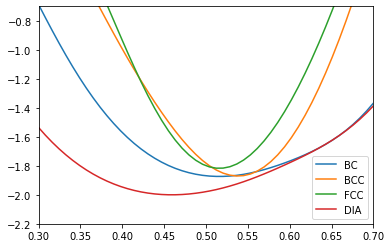
miniff is a minimal implementation of classical force fields: this tutorial demonstrates how to implement force fields for bulk Silicon. More exactly, we will reproduce Fig. 1 of Stillinger and Weber (1985) where they propose and benchmark a specific form of the classical potential.

The problem

Stillinger and Weber propose to use a sum of the following pair and a triple potentials to model chemical forces between atoms in Silicon, Eqs. 2.3 and 2.5.

\[f_2(r) = A ( B r^{-p} - r^{-q} ) \cdot \exp [(r - a)^{-1}]\]

\[f_3(r_1, r_2, \theta) = \lambda \exp [\gamma (r_1 - a)^{-1} + \gamma (r_2 - a)^{-1}] \times ( \cos \theta + \cos \theta_0 )^2\]

Fig. 1 presents how the sum of these potentials scales with atomic density for different types of cubic cells.

Computing with miniff

Stillinger-Weber potential form is readily available in miniff.potentials. To instantiate potentials we specify parameter values from the manuscript: A, B, p, q, a, λ, γ.

from miniff.potentials import sw2_potential_family, sw3_potential_family

si_gauge_a = 7.049556227
si_gauge_b = 0.6022245584
si_p = 4
si_q = 0
si_a = 1.8
si_l = 21
si_gamma = 1.2

sigma = 1  # length unit
epsilon = 0.5  # energy unit: fixes double counting

si2 = sw2_potential_family(
    gauge_a=si_gauge_a, gauge_b=si_gauge_b,
    a=si_a, p=si_p, q=si_q,
    epsilon=epsilon, sigma=sigma)

si3 = sw3_potential_family(
    l=si_l, gamma=si_gamma, cos_theta0=-1./3, a=si_a,
    epsilon=epsilon, sigma=sigma)

In addition, epsilon and sigma provide the energy and length scales, respectively. The second step is to construct unit cells with different symmetries: simple cubic (SC), body-centered cubic (BCC), face-centered cubic (FCC), and diamond. For this, we use kernel.Cell. We do not bother about lattice parameters for the moment: we will re-compute them from the density of atoms.

from miniff.kernel import Cell
import numpy as np

# simple cubic: one atom in a cubic box
c_sc = Cell(np.eye(3), np.zeros((1, 3)), ["si"], meta=dict(tag="BC"))

# BCC: one additional atom at the center of the box
c_bcc = Cell(np.eye(3), [[0, 0, 0], [.5, .5, .5]], ["si", "si"], meta=dict(tag="BCC"))

# FCC: three additional atoms at box face centers
c_fcc = Cell(np.eye(3), [[0, 0, 0], [.5, .5, 0], [.5, 0, .5], [0, .5, .5]],
    ["si"] * 4, meta=dict(tag="FCC"))

# diamond: rhombic unit cell with two atoms
c_dia = Cell([[0, 1, 1], [1, 0, 1], [1, 1, 0]], [[0, 0, 0], [.25, .25, .25]],
    ["si"] * 2, meta=dict(tag="DIA"))

cells = [c_sc, c_bcc, c_fcc, c_dia]

Finally, we apply a uniform strain to these cells and compute the total energy as a function of the atomic density. The kernel.profile_directed_strain batches multiple energy computations into a single function.

from miniff.kernel import profile_directed_strain
from matplotlib import pyplot

density = np.linspace(0.3, 0.7)  # target density values from the plot

for c in cells:
    d = c.size / c.volume  # actual density
    e = profile_directed_strain([si2, si3], c, (d / density) ** (1./3), (1, 1, 1))
    pyplot.plot(density, e / c.size, label=c.meta["tag"])

pyplot.ylim(-2.2, -0.7)
pyplot.xlim(0.3, 0.7)
pyplot.legend()

<matplotlib.legend.Legend at 0x7fcf331b8f50>

Tips

presentation.plot_strain_profile combines profile_directed_strain with plotting routines and constructs a similar figure.