Computing descriptors

Computing descriptors is an important part of both constructing datasets and using neural-network fits.

The problem

Consider a unit box in 3 dimensions. n = 100 atoms are present in the box; their cartesian coordinates are written in a [100 x 3] matrix r such that 0 <= r <= 1.

import numpy as np

n = 100
a = 0.3
r = np.random.rand(100, 3)

Our task is to count atomic neighbors inside a shell of size a = 0.3 for each atom. This is what a typical descriptor looks like: it counts neighbors in shells around each atom.

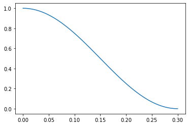
To make a continuous function out of neighbor count let’s introduce a kernel function of neighbor distance r smoothly decaying from a unit value at r = 0 down to zero at cutoff value r = a. Let’s take a half-period of cosine function for this example.

\[g(r) = \frac{1 + \cos \frac{\pi r}{a}}{2} \quad r < a\]

def g(r):
    return (1 + np.cos(np.pi * r / a)) / 2 * (r < a)

from matplotlib import pyplot
x = np.linspace(0, a)
pyplot.plot(x, g(x))

[<matplotlib.lines.Line2D at 0x7fc0cd9424d0>]

Instead of computing neighbors directly let’s compute the cumulative value of the kernel function for all neighbors.

\[n_i = \sum_j g (r_{ij})\]

Computing naively

We start with computing all pair distances between atoms.

mdist = np.linalg.norm(r[:, None, :] - r[None, :, :], axis=-1)

Then, we reduce pair distances using the kernel function.

result = g(mdist).sum(axis=0) - 1

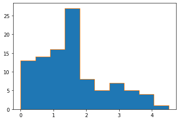
Finally, we can plot the distribution of neighbors across all points.

from matplotlib import pyplot
pyplot.hist(result)

(array([13., 14., 16., 27.,  8.,  5.,  7.,  5.,  4.,  1.]),
 array([0.        , 0.45074515, 0.90149029, 1.35223544, 1.80298058,
        2.25372573, 2.70447087, 3.15521602, 3.60596116, 4.05670631,
        4.50745146]),
 <BarContainer object of 10 artists>)

This approach is straightforward but not efficient. First, matrix mdist includes information about very distant atoms we simply discard. Second, we can only perform pair reductions this way: counting atomic triples within the same sphere of radius a will require a tensor with three dimensions raising memory requirements by a factor of n = 100. Instead, miniff uses a more efficient approach with a quasi-linear complexity scaling.

Computing neighbors with miniff

miniff provides an interface to computing neighbors efficiently. It uses KDTree from scipy to compute neighbor lists and cython functions to iterate over the list and to reduce it to the desired quantities. As such, there are two key steps.

1. Compute neighbor lists

The primary purpose of miniff.kernel module is to perform neighbor list construction using compute_images method and CellImages class. To do it, we first construct a unit cell object with atomic coordinates.

from miniff.kernel import Cell, compute_images

cell = Cell(np.eye(3), r, ['a'] * len(r))

The second step is to compute its images (neighbors) given the cutoff value and other periodicity information.

images = compute_images(cell, cutoff=a, pbc=False)
print(len(images.distances.data))

794

As a result, images.distances contains neighbor distance data.

2. Reduce

In principle, neighbor counts can be deduced from the sparse matrix images.distances directly with previously defined method g. A more conventional workflow is to pick a reduction function from miniff.potentials module. Specifically, miniff.potentials.sigmoid_descriptor_family provides the following reduction function:

\[n_i = \sum_j \frac{1}{1 + e^\frac{r_{ij} - r_0}{dr}} \cdot \frac{1 + \cos \frac{\pi r_{ij}}{a}}{2},\]

where r_ij is the distance matrix, r0, dr and a are constant parameters. By setting dr to a small value and r0 to 2a we simplify the expression to the second term only

\[n_i \approx \sum_j \frac{1 + \cos \frac{\pi r_{ij}}{a}}{2},\]

resembling the kernel above. To instantiate the descriptor we simply call the factory object the specified parameters.

from miniff.potentials import sigmoid_descriptor_family

descriptor = sigmoid_descriptor_family(r0=10 * a, dr=a / 10, a=a)

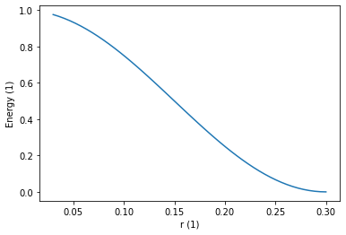
Let’s visualise the radial form of the descriptor.

from miniff.presentation import plot_potential_2

plot_potential_2(descriptor, energy_unit="1", length_unit="1")

<AxesSubplot:xlabel='r (1)', ylabel='Energy (1)'>

To perform the reduction we simply feed the descriptor to images.eval.

result_miniff = images.eval(descriptor.copy(tag="a-a"), "kernel")

Not that descriptor.copy(tag="a-a") makes a copy of the descriptor with the descriptor.tag = "a-a". The tag is required by images.eval to distinguish between species and possible pairs. For example, having two kinds of species in the box "a" and "b" we may reduce several kinds of pairs such as "a-a" or "a-b".

Additionally, we specify the function we want to compute. The same descriptor may provide multiple functions at once: "kernel" stands for the descriptor value while "kernel_gradient" efficiently computes descriptor gradients.

Finally, let’s plot and compare the result.

_, bins, _ = pyplot.hist(result)
pyplot.hist(result_miniff, bins, histtype="step")

(array([13., 14., 16., 27.,  8.,  5.,  7.,  5.,  4.,  1.]),
 array([0.        , 0.45074515, 0.90149029, 1.35223544, 1.80298058,
        2.25372573, 2.70447087, 3.15521602, 3.60596116, 4.05670631,
        4.50745146]),
 [<matplotlib.patches.Polygon at 0x7fc065414290>])

Advanced

miniff.potentials includes several most common reduction functions. But it is also possible to define yours using miniff.potentials.general_pair_potential_family. It accepts two methods: f(r) and df_dr(r). As f is a python function called multiple times during the reduction, it will not benefit from cython optimizations and parallelism. Nevertheless, it is a handy prototyping tool.