Toy function fitting¶

miniff is built around the idea of using neural-network fits to describe inter-atomic interactions. This is done in three basic steps:

constructing the dataset;
fitting the data (= finding optimal map parameters);
using the fit.

This tutorial demonstrates the first two steps in the context of simple scalar function fitting. We will pick a function and will try to perform a least-squares fit. Then, we will repeat the procedure with the help of miniff.ml and miniff.ml_util modules to introduce the key concepts of dataset construction and fitting in miniff.

The toy problem¶

Neural-network fitting is useful for interpolating black-box functions which otherwise require intensive computations. For pedagogical reasons, let us instead try to fit a simple analytic function defined for positive r and resembling some features of realistic interatomic potentials:

\[f \left ( r \right ) = \left ( r^2 - r + 1 \right ) e^{-r}.\]

Let’s first plot the function:

import numpy as np
from matplotlib import pyplot

def f(r):
    return (r ** 2 - r + 1) * np.exp(-r)

r = np.linspace(0.1, 10, 100)
f_r = f(r)
pyplot.plot(r, f_r)

[<matplotlib.lines.Line2D at 0x7f777a4ae4d0>]

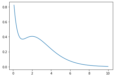
The function has two extrema at r = 1, 2 and decays rapidly: these are the features which we will attempt to reproduce.

When fitting, we only have access to discretized sampling values f_r, but not to the functional form f(r). In principle, we may still use f(r) as a black box to produce more sampling points but we consider this operation to be computationally expensive, thus, to only be used before the fitting.

1. Constructing the dataset¶

The fitting data (or the dataset) includes two pieces of information: blackbox outputs and descriptors. They can be also seen as right-hand and left-hand sides of the map g(r)->f(r) respectively, where f(r) are previously computed blackbox function values f_r.

What are descriptors?¶

The purpose of descriptors g(r) is to describe values of r where f(r) was computed in a physically reasonable way. Can we use values of g(r)=r directly? Yes, but g(r) play the role of pre-conditioners: we input some intuition about how f(r) would most reasonably look like while leaving particular details to be determined during the fitting process.

Additionally, we allow the blackbox function to have an arbitrary number of inputs such as

\[f \left ( \vec r \right ) = \sum_i { \left ( r_i^2 - r_i + 1 \right ) e^{-r_i}}.\]

In this case we may want to construct the dataset from vectors of a non-constant dimension r = ([0], [0.1, 0.2], [2.2, 3, 2], ...). To employ neural network machinery, however, we usually need a constant number of inputs. This can be achieved by using a descriptor of the form

\[g \left ( \vec r \right ) = \sum_i r_i\]

in place of r. Importantly, the above descriptor also respect the permutation symmetry of f(r): f(x, y) = f(y, x), g(x, y) = g(y, x). Thus, the follow-up fitting process does not need to deduce this symmetry in a hard way numerically.

How to choose descriptors?¶

g(r) should include as much intuition as possible (symmetries, asymptotic behavior, …);
g(r) should be simple enough functions fast to compute.

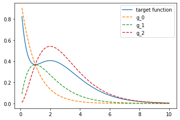
Here we choose the following family of descriptors which obviously satisfies both recommendations:

\[g_i (r) = r^i e^{-r}.\]

We also know the exact form of the map to be fitted:

\[f(r) = g_2(r) - g_1(r) + g_0(r).\]

So, to complete the dataset we compute g_0, g_1, g_2 at previously chosen sampling points.

def g(r, i):
    return r ** i * np.exp(-r)

g_r = np.array(tuple(g(r, i) for i in range(3)))
pyplot.plot(r, f_r, label="target function")
for i, _g in enumerate(g_r):
    pyplot.plot(r, _g, ls="--", label=f"g_{i}")
pyplot.legend()

<matplotlib.legend.Legend at 0x7f77498d4450>

2. Fitting the data¶

For this example whe know there exists a linear combination of descriptors perfectly reproducing the black-box function

\[f(r) = \sum_i a_i \cdot g_i(r).\]

Thus, the least-squares fit will find map parameters a_i.

gf_map, res, rank, s = np.linalg.lstsq(g_r.T, f_r)
print(gf_map)

from numpy import testing
testing.assert_allclose(gf_map, (1, -1, 1))

[ 1. -1.  1.]

According to the last formula in the previous section, the answer is [1, -1, 1].

miniff setting¶

The above solution can be also obtained from miniff with the same workflow.

1. Constructing the dataset (miniff)¶

miniff.ml contains handy pipelines for dataset construction and pre-processing. PerCellDataset and PerPointDataset are the two key containers where descriptors and target function values are stored. Some data pieces (such as descriptors, but also atomic charges and more) can be assigned to individual points (atoms) and are stored in PerPointDataset. Other data pieces (such as total interatomic energies) are cumulative values that are stored in PerCellDataset. Due to the nature of force-field fitting, there can be only one PerCellDataset but one or more ``PerPointDataset``s.

In this case we store f_r into the total interaction energy slot of PerCellDataset to benefit from the energy fitting pipeline.

import torch
from miniff import ml

rhs = ml.PerCellDataset(
    energy=torch.tensor(f_r, dtype=torch.float32)[:, None],
)

All dataset pieces have to be torch tensors of a fixed shape. In this case “energy” is required to be a column array with the second dimension equal to 1: otherwise a ValueError will be raised.

Descriptors are stored in PerPointDataset as a standard.

lhs = ml.PerPointDataset(
    features=torch.tensor(g_r.T, dtype=torch.float32)[:, None, :],
    mask=torch.ones(len(r), 1),
)

Here, we additionally specify the mask which weights individual data points. Again, the dimensions of input tensors are well-defined. As a final step, we collect the two pieces of fitting data into the Dataset object.

dataset = ml.Dataset(rhs, lhs)

At this point all tensor shapes are checked and we are ready to set up the fitting.

2. Fitting the data (miniff)¶

First, we need to define the functional form of the map. In this case the map is linear which can be declared using torch.nn.Linear.

\[f = W \cdot g,\]

where W stands for weights.

nn = torch.nn.Linear(in_features=3, out_features=1, bias=False)

Here, 3 stands for the descriptor count, 1 is output count (single energy), bias=False tells that no constant is added to the linear form.

To obtain the best fit we use energy fit optimisation pipeline defined in miniff.ml_util. First, we define the closure to be energy difference closure. In general, closure defines the loss function to optimize but the corresponding ml_util object also includes default optimization settings.

from miniff import ml_util

tolerance = dict(
    tolerance_change=1e-14,
    tolerance_grad=1e-14,
)

closure = ml_util.simple_energy_closure([nn], dataset,
    optimizer_kwargs=tolerance)

Let’s check that the initial (random) guess is non-optimal.

print("Initial loss:", closure.loss().loss_value.item())

Initial loss: 0.010355422273278236

Finally, let’s run the optimization and check the loss function value becomes small.

closure.optimizer_init()
closure.optimizer_step()  # LBFGS algorithm by default
loss = closure.last_loss.loss_value.item()
print("Final loss:", loss)
assert loss < 1e-8

Final loss: 1.784633621844346e-15

Parameters are now stored in the neural network module.

weights = nn.weight.detach().squeeze().numpy()
print(weights)
testing.assert_allclose(weights.squeeze(), [1, -1, 1], atol=1e-3)

[ 1.0000002 -1.0000002  1.0000001]

Checking the result¶

Finally, let’s check whether the fit is reasonable by plotting it.

def nn_fit(r, descriptor_fns, nn):
    # Compute descriptors
    descriptors = np.array(tuple(g(r) for g in descriptor_fns))
    # Compute the map
    result = nn(torch.tensor(descriptors.T, dtype=torch.float32))
    return result.detach().numpy().squeeze()

from functools import partial

f_r_test = nn_fit(
    r,
    tuple(partial(g, i=i) for i in range(3)),
    nn,
)
pyplot.plot(r, f_r)
pyplot.scatter(r, f_r_test)

<matplotlib.collections.PathCollection at 0x7f76dffe0c50>

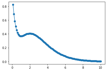
The function nn_fit demonstrates how to propagate the map forward: one needs to (1) compute descriptors as a function of input r and (2) to feed them to the neural network.

Advanced¶

It does not make sense to use anything but linear map for this particular problem with a known exact solution. However, if we chose to, for example, reduce the descriptors to g_0 only or to chose different descriptors then the linear map becomes a crude approximation. In this case one typically switches to a more general neural-network setting with non-linear activation layers helping to map various curvature features in the dataset. One can use torch machinery for this or just otherwise increase n_layers when initializing the map. With n_layers=2, for example, one sigmoid activation layer is inserted between two linear layers.

The use of ml_util functions is entirely optional. They aim to provide default optimization setting to start with: loss functions (2-norm), optimizers (LBFGS), descriptor sets (Behler recipe). You are free to modify and replace these components at the point when you feel that the default choice is no longer optimal.